Creating an illustration like image from photos
In the 1980s, when I became a company employee from a university student, the illustration drawn by Eizin Suzuki were beautiful and very popular in Japan. HERE is the link to Eizin Suzuki's official site.
His illustration are so impressive that I often want to turn photos taken by myself into the pictures like his works. I believe that it should be possible to create even professional images like this using Adobe software or the software such as GIPM, so I have tried it several times. However, the operation of the software, say using layers, is complicated for me, and so I gave up every time getting frustrated even within an hour.
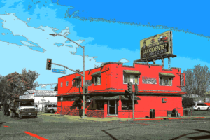
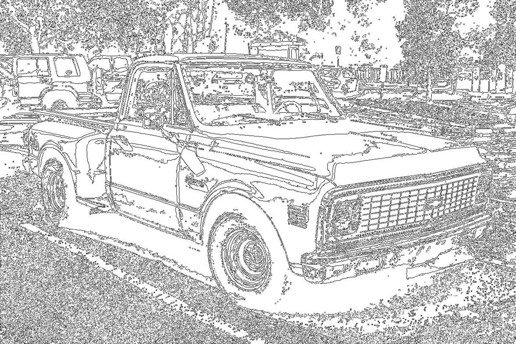
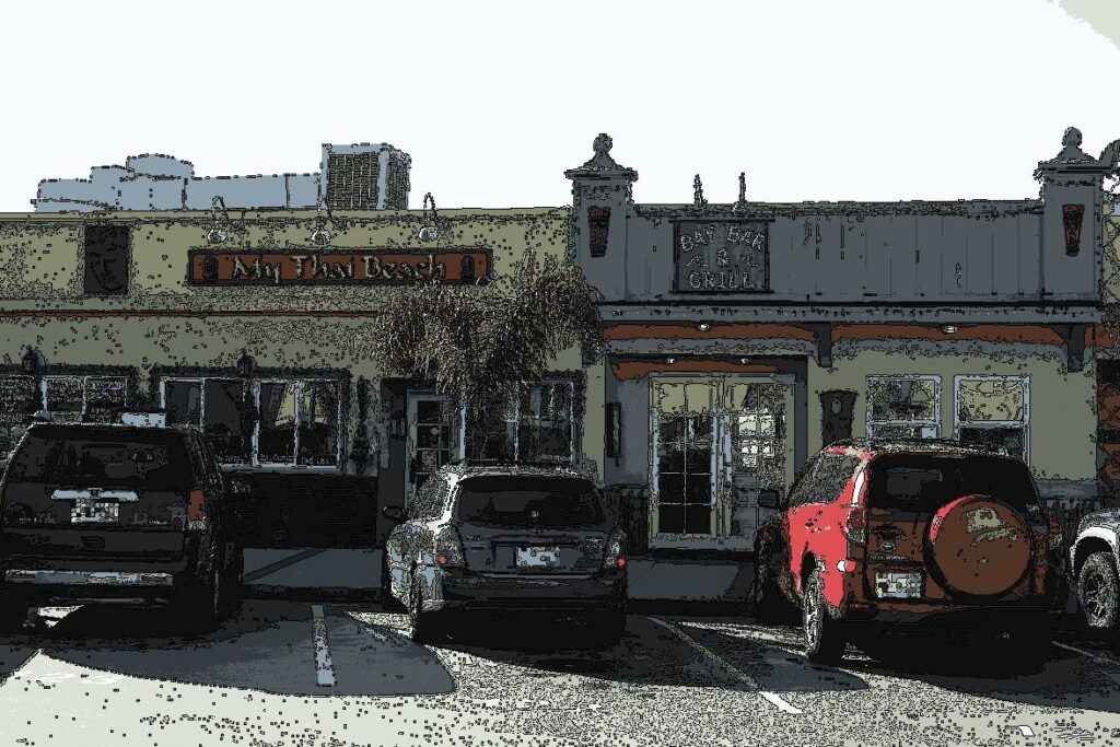
When I am doing image processing, in the meantime, I realize that I could get similar images, if I group similar color tones together by dimensionality reduction, calculate the boundaries of the images after that, and put them together. I tried it here using K-means clustering for dimensionality reduction, Canny for edge detection. The results went well like this.
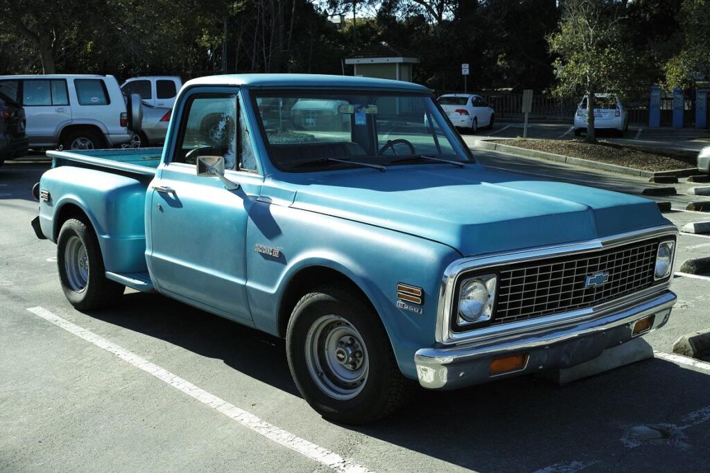
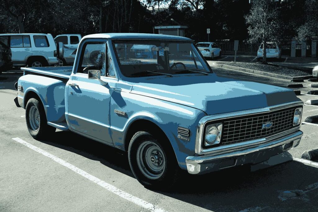
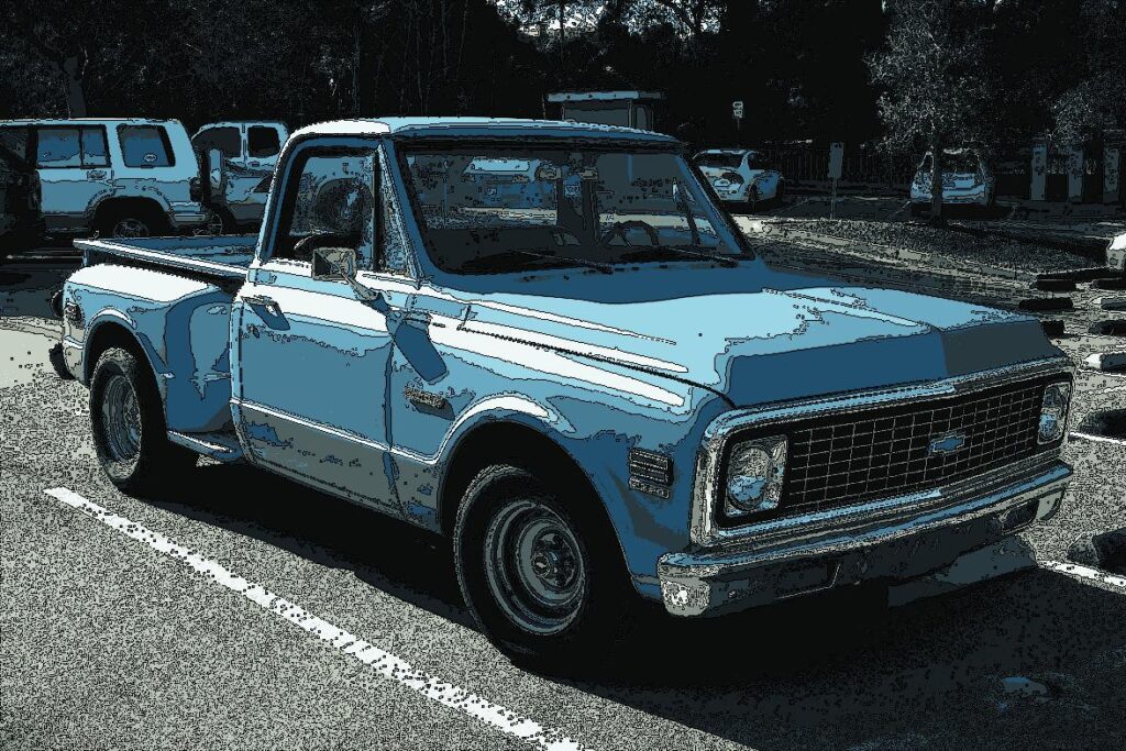
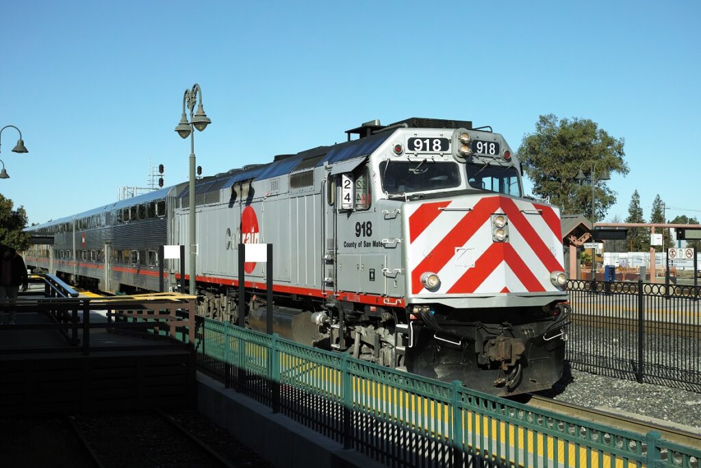
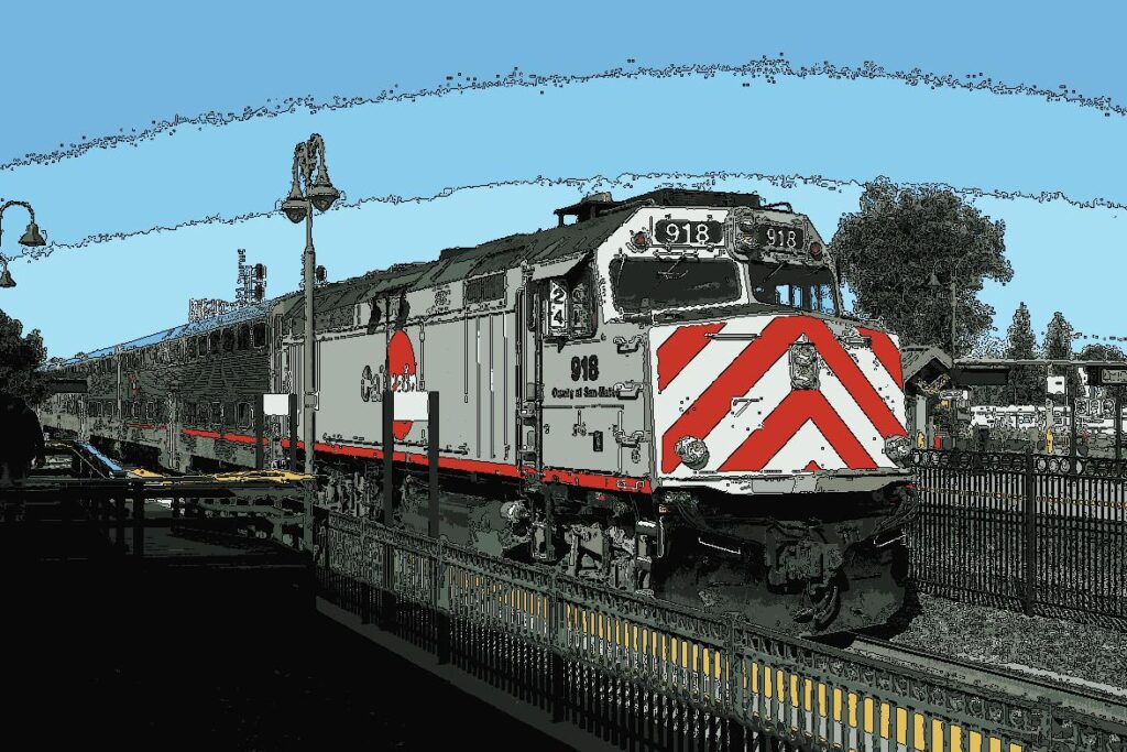
With a very short code I think I succeeded in creating a similar taste illustration. However, the color vibrancy falls far short. Next time, I would like to try color adjustment. Here are some other photos applying the code.

Code
# import libraries

import numpy as np                                 # import libraries
import cv2
import matplotlib.pyplot as plt
from sklearn.cluster import KMeans
%matplotlib inline

# load an image and compress colors
img = plt.imread('data/2016_Bay_Area_1_00.jpg')     # load an image
img_s = img / 255                                   # scaling

img_s_pre_clusteing = img_s.reshape(img.shape[0] * img.shape[1], 3)     # reshape for clustring
k_means = KMeans(12)                                                    # apply K-means
k_means.fit(img_s_pre_clusteing)

img_d_reduction = k_means.cluster_centers_[k_means.labels_].reshape(img.shape[0], img.shape[1], 3)      # image color compressed

# compare the original and color compressed image and save the images
fig = plt.figure(figsize = (22, 10))
ax1 = fig.add_subplot(1, 2, 1)
ax2 = fig.add_subplot(1, 2, 2)

ax1.imshow(img)
ax2.imshow(img_d_reduction)

plt.imsave('data/original_image.jpg', img)
plt.imsave('data/dimension_reduction_image.jpg', img_d_reduction)
plt.show()

image = (255 * (0.299 * img_d_reduction[:, :, 0] + 0.587 * img_d_reduction[:, :, 1] + 0.114 * img_d_reduction[:, :, 2]))    # convert to a gray image
image = (image * 255).astype(np.uint8)     # change the data type

# edge detection
canny_image = cv2.Canny(image, 50, 100)          # Canny edge detection
canny_image_r = cv2.bitwise_not(canny_image)     # reverse black and white

plt.figure(figsize = (20, 10))
plt.imsave('data/edge_detection_image.jpg', canny_image_r, cmap = 'gray')
plt.imshow(canny_image_r, cmap = 'gray')
plt.show()

# overlap the image with dimension reduction and edges
for i in range(canny_image_r.shape[0]):
    for j in range(canny_image_r.shape[1]):
        for k in range(3):
            if canny_image_r[i, j] == 0:
                img_d_reduction[i, j, k] = 0

# see the final image
plt.figure(figsize = (20, 10))
plt.imshow(img_d_reduction)
plt.imsave('data/final_image.jpg', img_d_reduction)
plt.show()
The code is downloadable from the link below. This operation is another exercise for me. Even if you like it, use at your own risk.